Data Clustering - Clustering two-dimensional (2D) data
(Last modified: 05 Oct 2017, 14:49)
Introduction
In this post, we will show a simple example of clustering data in two dimensions. As usual, we will try to keep terminology and ideas as simple as possible.
Data clustering is the partitioning of data into a number of clusters such that all data within a given cluster are similar to each other and dissimilar to data in other clusters. A metric is normally used as the criterion for data clustering and one of the most popular is the distance metric, where data within a cluster are closer to each other and further from data in other clusters.
The clustering of the data is achieved using clustering algorithms which usually work in an interative fashion. In each iteration, the algorithms assigns the data to different clusters with the objective of minimizing the sum of square error (SSE) between a data point and the assigned mean of its assigned cluster.
There are many clustering algorithms (see References) we will restrict our discussion to two of the more popular clustering algorithms are k-means (hard) and c-means (fuzzy) clustering algorithms.
After the clustering, each data point is assigned a membership value (for each cluster) which determines its probability of membership in that cluster. For k-means clustering algorithm, the membership values are discrete and are either 0 or 1, i.e., a data point is either in a cluster or not. For fuzzy (or c-means) clustering algorithm, the membership values varies between 0 and 1, which means that a data point has membership, to varying degrees, in all the clusters. In the c-means case, the membership values are constraint but constrained to sum to 1.
Unless stated otherwise, we perform the clustering using c-means algorithm and references to clustering refers to this variant.
We illustrate the clustering using simple synthetic data in two dimensions. This will allow us to show the results of our clustering in 2D/3D plots. However, clustering can be applied to high-dimensional data much greater than 2.
In subsequent post, we will consider more complex data sets and data from public domain, e.g., the Iris Data Set and similar data sets hosted at the UCI Machine Learning Repository.
I am using a simple script that implements fuzzy clustering algorithm. Many data analysis software and tools (R, Matlab, Python, etc) have packages and/or built tools for data clustering.
Synthetic Data
For our clustering example, we will use a synthetical data with the following assumptions:
1 Number of data points: We assume two-dimensional data and each data point has exactly two attribute values, its X and Y values. The number of data points is set at 400.
2 Number of clusters: The correct number of clusters in the data set is assumed to be known.
To perform clustering, we normally specify the number of clusters as an input to clustering algorithm. For the examples presented here, the correct number of clusters is known. This is usually not the case for practical data which are usually large (number of samples) and high-dimensional (number of attributes/features). These data can not be visualized as a whole but slices of the data (sets of attributes) can be visualized in 2D/3D plots. There are workflows for determining the optimal number of clusters for such data and will consider an example workflow in a subsequent post.
Using a simple script, I generated two sets of sample data. In Sample 1 (see Figure 1), there are four clusters that are clearly separate. This case is trivial but we will use it to prove that our clustering of the data is correct i.e., all data are assigned to the correct clusters.
We will illustrate the correctness of the clustering by plotting the membership values of the data points. For this simple tests, we have tried to make sure that the clusters are of the same shape (spherical) and contain about the same number of data points. In a subsequent post, we will look at differently shaped clusters, e.g., elongated and spherical.
The Sample 2 data set (see Figure 2) is similar to Sample 1 in that it was generated with 4 clusters, but now, the clusters are not as clearly separated as those in Sample 1.
Sample 1 Clustering Results
The results of clustering data Sample 1 are shown in Figures 3 and 4. The figures are three dimensional plot with the cluster membership values on the Z-axis and the data point on the X- and Y-axis respectively. Figure 3 shows the raw cluster membership values as obtained from the clustering. Each data point has a membership value in all the clusters.
In general, the farther a data point is from other cluster, the smaller it’s membership value in that cluster. In our example, where the clusters are clearly separated, the membership of a given data will be high for the cluster it belongs and low for the other cluster. For example, the membership values for the first data point is shown in Table 1.
From Table 1, we observe that the first data point has a higher likelihood of belonging to cluster 2. The assigment of other data points to clusters follows the same ideas. Note that the membership functions usually sums to 1.0.
Figure 2(b) presents the same information after hardening the membership values. This means that we find the highest membership value and set it to 1.0 and then we set the others to a value of zero. For the first data point, the membership values after hardening is shown in Table 2
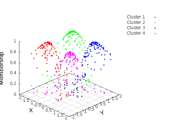
Sample 2 Clustering Results
We performed the same analyses on Sample 2 and obtained the cluster membership plots shown in Figures 3 and 4 with each cluster assigned a different color. In Figure 3, we observe that points that are in the middle of the cluster, i.e., closer to the cluster centroid, have higher membership functions than points that are located at the edge of the clusters. Also, there is a decrease in the membership function values as we move from the center of the clusters towards the edge, hence the inverted bowl effect.
Figure 4 shows the hardened membership function values for the four clusters. As described earlier, hardening converts the membership values to values that are either 0 or 1, i.e., the highest membership value is set to a value of 1 and the others set to 0.
Conclusion
We have describe an example of (fuzzy) clustering of synthetic two-dimensional data with spherical cluster shapes. We showed that the clustering algorithm is able to assign each data point to the correct cluster based on the data membership values. This is expected because we know the number of clusters in our data and this was specified as input to the clustering algorithm. In practice, we do not know the number of clusters and other iterative workflow will be used to determine the optimal number of clusters in the data. We will show this in a future post.
In these examples, we considered 2d data, however, clustering can be performed in much higher dimensions (d>2). In our next post, we will take a look at a real data set from the UCI Machine Learning Repository.
References
There are many good references on clustering and clustering algorithms. Here I have listed a few including a book, and several orders listed in the Princeton and Wikipedia pages. I will update the reference list to include other resources.
- Richard O. Duda, Peter E. Hart, David G. Stork (2001). Pattern classification (2nd ed.). Wiley, New York. ISBN 0-471-05669-3
- https://www.cs.princeton.edu/courses/archive/fall08/cos436/Duda/PR_refs.htm
- https://en.wikipedia.org/wiki/Pattern_recognition